话不多说就开始吧!
1
2
3
4
5
6
import pandas as pdgapminder = pd.read_csv('gapminder.csv' ) print(type(gapminder)) gapminder.head()
<class 'pandas.core.frame.DataFrame'>
country
continent
year
lifeExp
pop
gdpPercap
0
Afghanistan
Asia
1952
28.801
8425333
779.445314
1
Afghanistan
Asia
1957
30.332
9240934
820.853030
2
Afghanistan
Asia
1962
31.997
10267083
853.100710
3
Afghanistan
Asia
1967
34.020
11537966
836.197138
4
Afghanistan
Asia
1972
36.088
13079460
739.981106
(1704, 6)Index(['country', 'continent', 'year', 'lifeExp', 'pop', 'gdpPercap'], dtype='object')RangeIndex(start=0, stop=1704, step=1)<class 'pandas.core.frame.DataFrame'>
RangeIndex: 1704 entries, 0 to 1703
Data columns (total 6 columns):
country 1704 non-null object
continent 1704 non-null object
year 1704 non-null int64
lifeExp 1704 non-null float64
pop 1704 non-null int64
gdpPercap 1704 non-null float64
dtypes: float64(2), int64(2), object(2)
memory usage: 80.0+ KB
year
lifeExp
pop
gdpPercap
count
1704.00000
1704.000000
1.704000e+03
1704.000000
mean
1979.50000
59.474439
2.960121e+07
7215.327081
std
17.26533
12.917107
1.061579e+08
9857.454543
min
1952.00000
23.599000
6.001100e+04
241.165877
25%
1965.75000
48.198000
2.793664e+06
1202.060309
50%
1979.50000
60.712500
7.023596e+06
3531.846989
75%
1993.25000
70.845500
1.958522e+07
9325.462346
max
2007.00000
82.603000
1.318683e+09
113523.132900
数据整理
dplyr的基本功能是六个能与SQL查询语法相互呼应的函数:
filter()函数:SQL查询中的where描述
select()函数:SQL查询中的select描述
mutate()函数:SQL查询中的衍生字段描述
arrange()函数:SQL查询中的order by描述
summarise()函数:SQL查询中的聚合函数描述
group_by()函数:SQL查询中的group by描述
1 2 3 gapminder[gapminder['country' ] == 'China' ]
country
continent
year
lifeExp
pop
gdpPercap
288
China
Asia
1952
44.00000
556263527
400.448611
289
China
Asia
1957
50.54896
637408000
575.987001
290
China
Asia
1962
44.50136
665770000
487.674018
291
China
Asia
1967
58.38112
754550000
612.705693
292
China
Asia
1972
63.11888
862030000
676.900092
293
China
Asia
1977
63.96736
943455000
741.237470
294
China
Asia
1982
65.52500
1000281000
962.421380
295
China
Asia
1987
67.27400
1084035000
1378.904018
296
China
Asia
1992
68.69000
1164970000
1655.784158
297
China
Asia
1997
70.42600
1230075000
2289.234136
298
China
Asia
2002
72.02800
1280400000
3119.280896
299
China
Asia
2007
72.96100
1318683096
4959.114854
1 2 gapminder[(gapminder['year' ] == 2007 ) & (gapminder['continent' ] == 'Asia' )].iloc[0 :10 ,]
country
continent
year
lifeExp
pop
gdpPercap
11
Afghanistan
Asia
2007
43.828
31889923
974.580338
95
Bahrain
Asia
2007
75.635
708573
29796.048340
107
Bangladesh
Asia
2007
64.062
150448339
1391.253792
227
Cambodia
Asia
2007
59.723
14131858
1713.778686
299
China
Asia
2007
72.961
1318683096
4959.114854
671
Hong Kong, China
Asia
2007
82.208
6980412
39724.978670
707
India
Asia
2007
64.698
1110396331
2452.210407
719
Indonesia
Asia
2007
70.650
223547000
3540.651564
731
Iran
Asia
2007
70.964
69453570
11605.714490
743
Iraq
Asia
2007
59.545
27499638
4471.061906
1 2 gapminder[['country' , 'continent' ]].iloc[0 :10 ,]
country
continent
0
Afghanistan
Asia
1
Afghanistan
Asia
2
Afghanistan
Asia
3
Afghanistan
Asia
4
Afghanistan
Asia
5
Afghanistan
Asia
6
Afghanistan
Asia
7
Afghanistan
Asia
8
Afghanistan
Asia
9
Afghanistan
Asia
1 2 3 4 gapminder['country_abb' ] = gapminder['country' ].apply(lambda x: x[:3 ]) gapminder.iloc[1 :10 ,]
country
continent
year
lifeExp
pop
gdpPercap
country_abb
1
Afghanistan
Asia
1957
30.332
9240934
820.853030
Afg
2
Afghanistan
Asia
1962
31.997
10267083
853.100710
Afg
3
Afghanistan
Asia
1967
34.020
11537966
836.197138
Afg
4
Afghanistan
Asia
1972
36.088
13079460
739.981106
Afg
5
Afghanistan
Asia
1977
38.438
14880372
786.113360
Afg
6
Afghanistan
Asia
1982
39.854
12881816
978.011439
Afg
7
Afghanistan
Asia
1987
40.822
13867957
852.395945
Afg
8
Afghanistan
Asia
1992
41.674
16317921
649.341395
Afg
9
Afghanistan
Asia
1997
41.763
22227415
635.341351
Afg
1 2 gapminder[gapminder['year' ] == 2007 ][['pop' ]].sum()
pop    6251013179
dtype: int64
1 2 gapminder[gapminder['year' ] == 2007 ][['lifeExp' , 'gdpPercap' ]].mean()
lifeExp 67.007423
gdpPercap 11680.071820
dtype: float641 2 gapminder[gapminder['year' ] == 2007 ].groupby(by = 'continent' )['pop' ].sum()
continent
Africa 929539692
Americas 898871184
Asia 3811953827
Europe 586098529
Oceania 24549947
Name: pop, dtype: int641 2 gapminder[gapminder['year' ] == 2007 ].groupby(by = 'continent' )['lifeExp' , 'gdpPercap' ].mean()
lifeExp
gdpPercap
continent
Africa
54.806038
3089.032605
Americas
73.608120
11003.031625
Asia
70.728485
12473.026870
Europe
77.648600
25054.481636
Oceania
80.719500
29810.188275
Python可视化的基石是Matplotlib套件的pyplot,她的绘图哲学是将图形的元素,例如坐标轴、线、点或者文字用不同的方法一一拼凑起来,优点是绘图的弹性非常高,缺点则是对于初学者的门坎略高。为了解决这个问题,pandas套件将matplotlib.pyplot的基础图形包装起来成为一个方法,让使用者只要呼叫df.plot()就能够便利地绘图,可以选择的图形种类相当丰富,只要指定kind =参数即可:
1 2 3 4 5 6 7 8 9 import matplotlib.pyplot as pltimport seaborn as snsgapminder_cn = gapminder[gapminder['country' ] == 'China' ] gapminder_cn[['year' , 'pop' ]].plot(kind = 'line' , x = 'year' , y = 'pop' , title = 'Pop vs. Year in China' ) plt.show()
1 2 3 4 5 6 gapminder_northasia = gapminder.loc[gapminder['country' ].isin(['China' , 'Japan' , 'Korea, Rep.' ])] gapminder_northasia_pivot = gapminder_northasia.pivot_table(values = 'lifeExp' , columns = 'country' , index = 'year' ) gapminder_northasia_pivot.plot(title = 'Life Expectancies in North Asia' ) plt.show()
1 2 3 4 5 6 gapminder_2007 = gapminder[gapminder['year' ] == 2007 ] gapminder_2007[['pop' , 'gdpPercap' , 'lifeExp' ]].hist(bins = 15 ) plt.show()
1 2 3 gapminder_2007[['gdpPercap' ]].plot(kind = 'hist' , title = 'GDP Per Capita in 2007' , legend = False , bins = 15 ) plt.show()
1 2 3 4 gapminder_continent_pivot = gapminder_2007.pivot_table(values = 'gdpPercap' , columns = 'continent' , index = 'country' ) gapminder_continent_pivot.plot(kind = 'hist' , alpha=0.5 , bins = 20 , title = 'GDP Per Capita by Continent' ) plt.show()
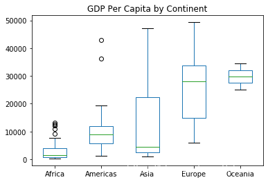
1 2 3 gapminder_continent_pivot.plot(kind = 'box' , title = 'GDP Per Capita by Continent' ) plt.show()
1 2 3 4 5 6 gapminder_2007.plot(kind = 'scatter' , x = 'gdpPercap' , y = 'lifeExp' , title = 'Wealth vs. Health in 2007' ) plt.show() gapminder_2007.plot(kind = 'hexbin' , x = 'gdpPercap' , y = 'lifeExp' , title = 'Wealth vs. Health in 2007' , gridsize = 20 ) plt.show()
1 2 3 4 5 summarized_df = gapminder[gapminder['year' ] == 2007 ].groupby(by = 'continent' )['pop' ].sum() summarized_df.plot(kind = 'bar' , rot = 0 ) plt.show()
1 2 3 4 5 6 7 8 9 10 11 12 13 14 15 mean_df = gapminder[gapminder['year' ] == 2007 ].groupby('continent' )['lifeExp' ,'gdpPercap' ].mean() mean_df = mean_df.reset_index() mean_df.head() fig = plt.figure() ax = fig.add_subplot(111 ) ax.plot(mean_df['continent' ], mean_df['lifeExp' ], '-' , label = 'lifeExp' ) ax2 = ax.twinx() ax2.plot(mean_df['continent' ], mean_df['gdpPercap' ], '-r' , label = 'gdpPercap' ) ax.set_ylim(40 ,100 ) ax2.set_ylim(0 , 50000 ) ax.legend(loc='upper left' ) ax2.legend(loc='upper right' ) plt.show()
Author:
SiQing
License:
Copyright (c) 2019 CC-BY-NC-4.0 LICENSE